home..

Raymarched Water

Nathan Reilly / January 2026 (3937 Words, 22 Minutes)

blizzardgame

Goal

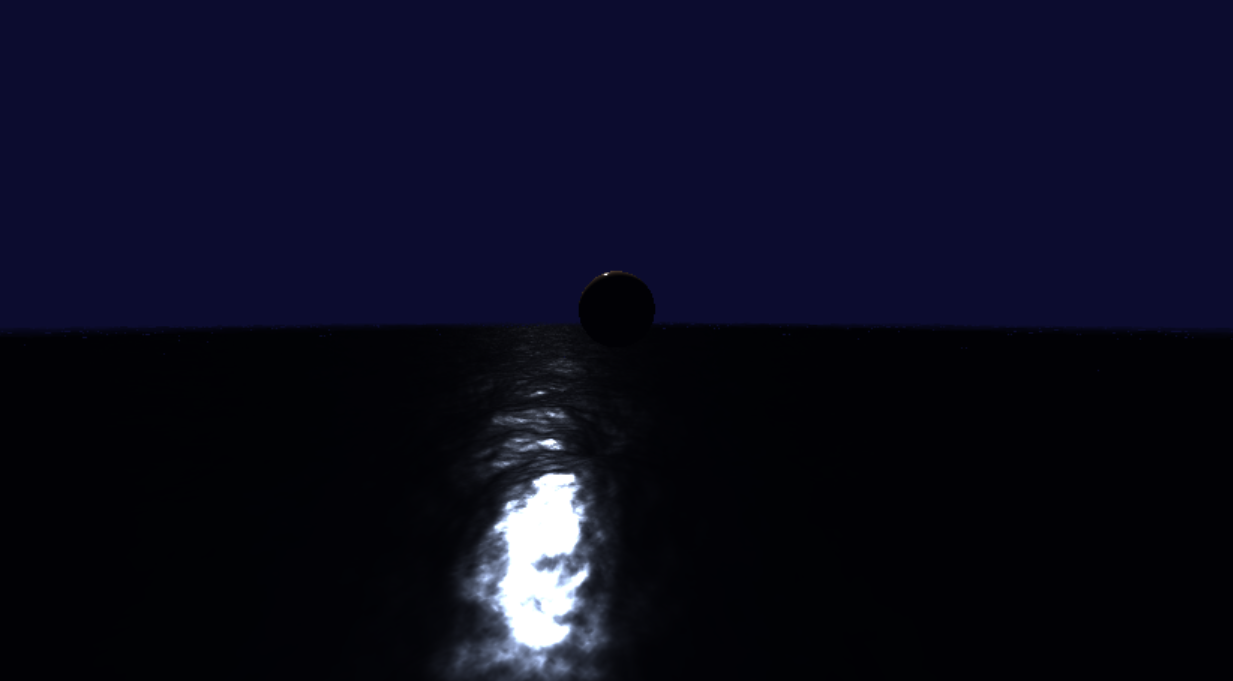
The overall goal of this mini-project is to render something that looks convincingly like the ocean. This will include realistic water lighting that is ideally adaptable to wave dynamics, in addition to a realistic simulation of the ocean waves themselves. In the end, it should look something like this:

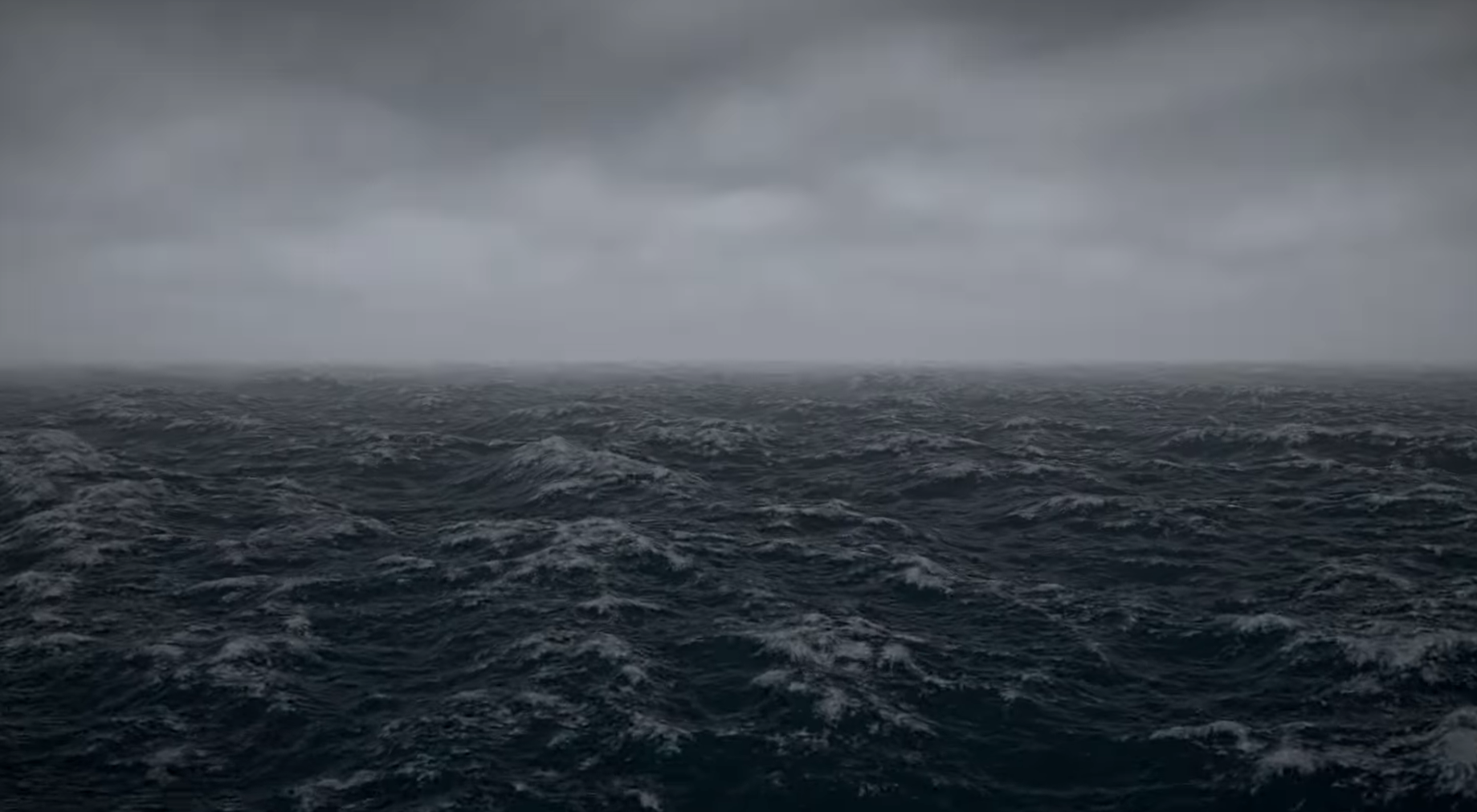Taken from the youtube video “Ocean waves simulation with Fast Fourier transform” by Jump Trajectory

The inspiration for this project came when learning about common strategies for rendering water, and then through further research, finding out about Fast Fourier Transforms. I did a dive into how Fourier Transforms work, and I felt that I had enough understanding to try and implement an FFT ocean simulation myself. I’m also a huge fan of Sea of Thieves, a game with some of the best water rendering out there, and wanted to try and imitate what they were able to accomplish.

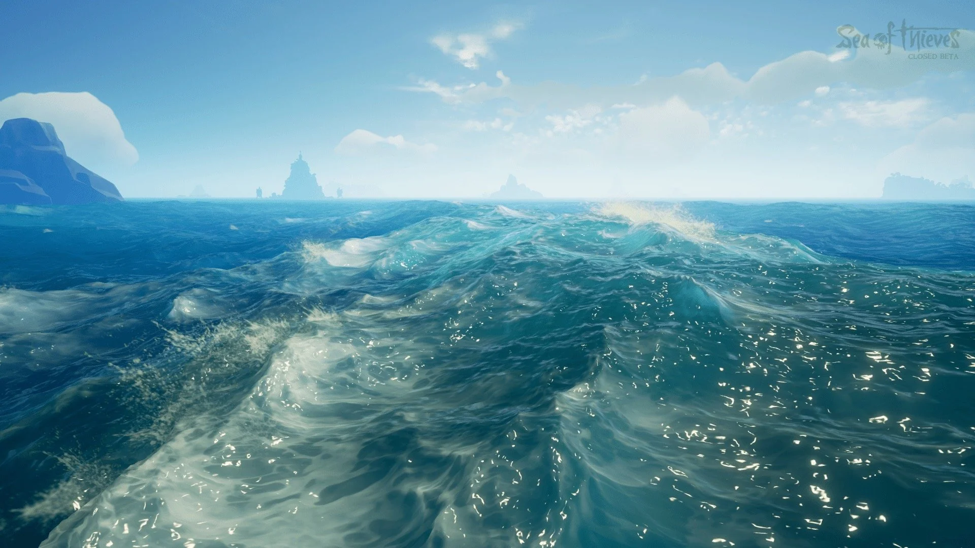Water from Sea of Thieves (Source)

The Tool

Before I could start working on this project, I of course needed to decide on the means to the end. That is, what will I use to create this ocean render?

For small graphics rendering projects like these, a common choice is Shadertoy. This is a website where you can write standalone fragment shaders. Briefly described, shaders are essentially just programs that run on the GPU. Fragment shaders specifically run once per pixel. The shader itself takes the pixel position as input, and outputs the color to be drawn at that pixel.

Note Shadertoy actually has many other posted successful attempts of what I aim to do, e.g. see below. However, I’ve decided to avoid looking at existing implementations, and try and figure out an implementation on my own using existing techniques and math that I find. It’d be too easy (and not educational enough) if I just copied someone else.

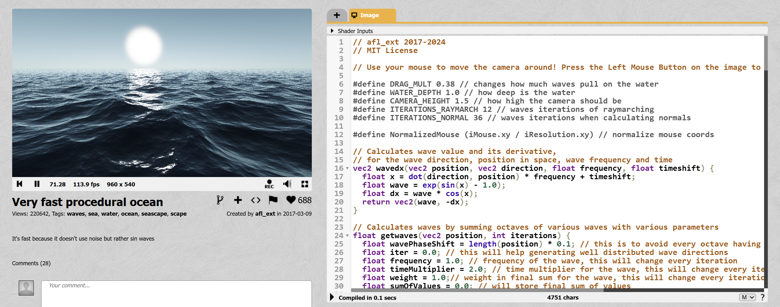An existing ocean render on Shadertoy, Source

Turns out, to render even complex scenes like these, this is all we actually need tool-wise. However, instead of Shadertoy, I’ll be using Posh Brolly. This is a very similar website, though it holds a more modern UI design, and a nice built-in movable camera.

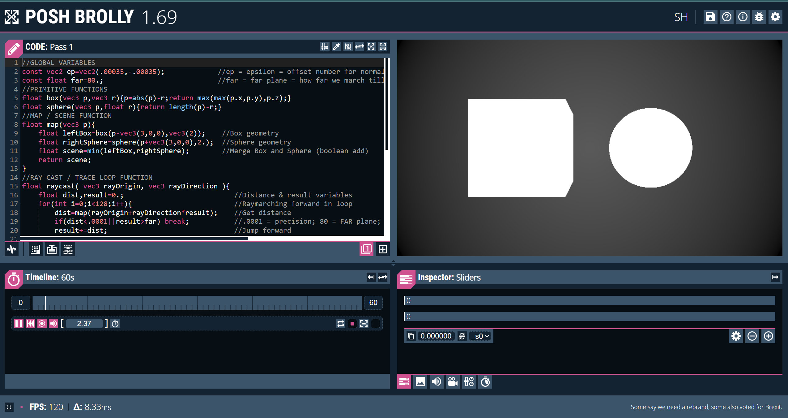Screenshot of the Posh Brolly editor interface

Raymarching

Rasterization - The Usual Way

If you have experience in 3D graphics, you may be aware that the most common way to render scenes in real-time applications (e.g. video games) is rasterization.

Briefly, rasterization as a technique renders a scene by taking a list of 3D points (called vertices) that each describe the corners of some triangle. It then determines where this triangle should be drawn on the screen, and then draws it there.

But how do we “draw it there”? Basically, given the three corners of some triangle in the scene, we can mathematically determine exactly which pixels it overlaps with. Then, for each of those pixels, we draw a specific color. That is, the color we want that triangle to be.

This is of course oversimplified, and there is much more customization and nuances to these steps, but that’s the gist of it.

Everything in the scene is essentially built up of thousands (or, for intensive games, millions) of small triangles. With so much detail, it ends up looking pretty realistic. 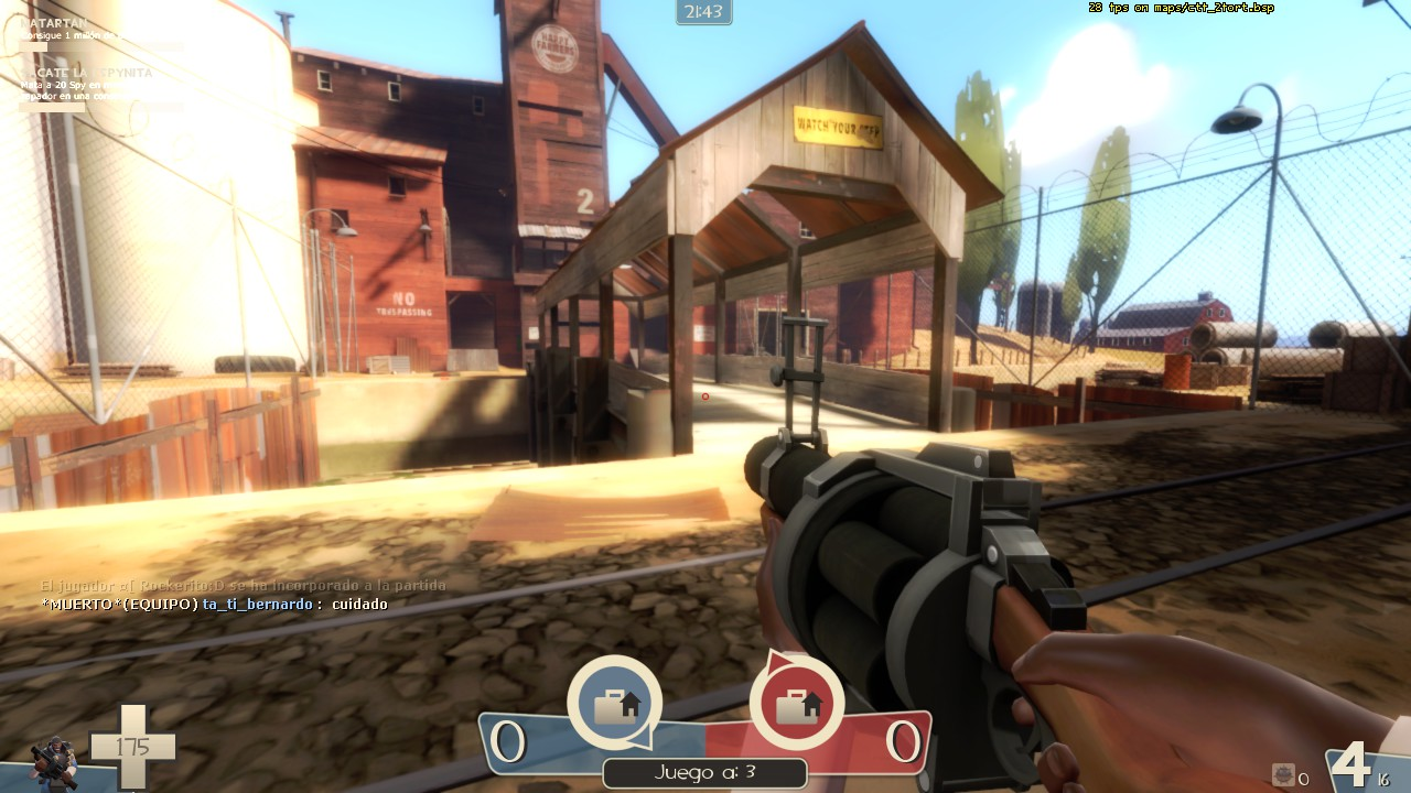A rasterized scene from Team Fortress 2, a video game.

The advantage that rasterization has over other techniques is that it is relatively fast, and optimized to run in parallel, something the GPU loves. So, this is by far the most common technique for any real-time rendering application.

In practice, rasterization requires the use of the entire graphics pipeline. That is, you’ll at least have a vertex shader which determines the vertices (i.e. the triangle corners), and the fragment shaderthat determines the color of each pixel within the triangles formed by those vertices. For our case, however, we only have access to the fragment shader stage, and it runs for every pixel on the screen instead of only for those within specific triangles.

Raymarching - The Fragment-Only Way

Background

So, what do you do when you only have a fragment shader? That’s where raymarching comes in.

In Posh Brolly (and of course Shadertoy), we are in control of a fragment shader that runs once for each pixel on the screen. In this context, we can in fact think of it as us simply having control of a program that takes pixel position as input, and must give pixel color as output.

To illustrate this, take the example of Posh brolly’s Cardboard Sandwich template shader:

const float PI=3.14159265359;
void mainImage(out vec4 fragColor,in vec2 fragCoord){
    vec2 uv=(fragCoord/_res-0.5)/vec2(_res.y/_res.x,1);  //2d uvs
    vec3 col=vec3(0.5)*cos(uv.x*PI)*.5+.5;
    fragColor=vec4(col,1);
}

Notice the mainImage function’s signature. It takes in a 2D vector called fragCoord, and outputs a 4D vector called fragColor. This is exactly what we would expect.

fragCoord is the position of our pixel in normalized device coordinates. That is, the bottom left corner is \((0,0)\), the top left is \((1,1)\), and all other pixel coordinates are interpolated in between.

fragColor is the color that we set to our pixel. It is in RGBA format, and thus is represented as a 4D vector, i.e \((r,g,b,a)\).

Our job is to use the value of fragCoord to determine the value of fragColor. We also get some useful things like the screen’s resolution _res and the time elapsed _t, which we will also use.

Using Raymarching

Raymarching allows us to use only the pixel’s location to choose the color we want, which is exactly the kind of technique we need. But how does it work?

Note this is a simplified explanation, but captures the essence of what’s going on. See this video by Sum and Product for a very good and more in-depth explanation.

Marching the Ray

You’ve likely heard of raytracing, and raymarching itself is conceptually very similar. In essence, it renders the scene by asking the question: What object is “behind” this pixel?. Of course, the answer to that question will tell us what color that pixel should be.

To do so, you consider the camera itself (i.e. you) to be an infinitely small point, and the screen to be a sort of window that it looks through. For each “pixel” of this window, a ray is marched from the camera’s exact position, through that pixel, and then continuing in that same direction until it “hits” an object in the scene. 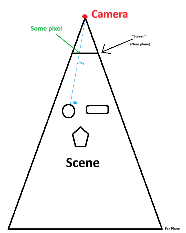2D raymarching visualization

The “marching” process in raymarching refers to the way that this ray moves forward. In essence, the ray’s position starts at the camera and then moves along the intended direction (through the pixel and beyond) in discrete steps. It continues to do so until it either gets close enough to some object, or too far from the camera (i.e. past the far plane). If it gets close enough to an object, we consider it a “hit” on that object. We then say that the pixel the ray travelled through should contain that object’s color, and voila, a rendered scene.

Though, from here, two open questions remain:

At each discrete step, how do we know how large of a step to take? That is, how much distance should we travel along the intended direction.
How do we know if we are “close enough” to an object?

Both of these questions are addressed by the use of signed distance functions (SDFs).

The Signed Distance Function

In a raymarched scene, each object has an associated SDF. This SDF takes a 3D position as input, and tells you how far that 3D position is from the associated object.

For example, if I have a sphere, I can calculate my distance to that ball with the following function:

// Calculates the distance from 'position' to the sphere centered at
//   'sphere_position' with radius 'radius'
float sdf_sphere(vec3 position, vec3 sphere_position, float radius) {
	float distance_to_center = length(sphere_position - position);
	return distance_to_center
}

Now let’s say I am at some point in the scene, and I want to know how far I am from the closest object to me. To get this value, I can give my 3D position to the SDF of each object in the scene, and this will provide me a list of distances to each object. Then, I can take the minimum of all of these distances, and that value will be my desired result; that is, the distance to the closest object.

This is the key to determining how large of a step our ray should take. In fact, that value is the step size.

Note that, for each discrete step, we want our ray to move as far as possible. At the same time, however, we also want to avoid overshooting an object (i.e. marching through it), as this would make it invisible.

So, if we know that no object is closer than some distance value, this gives us the largest possible amount of distance we can safely cover. 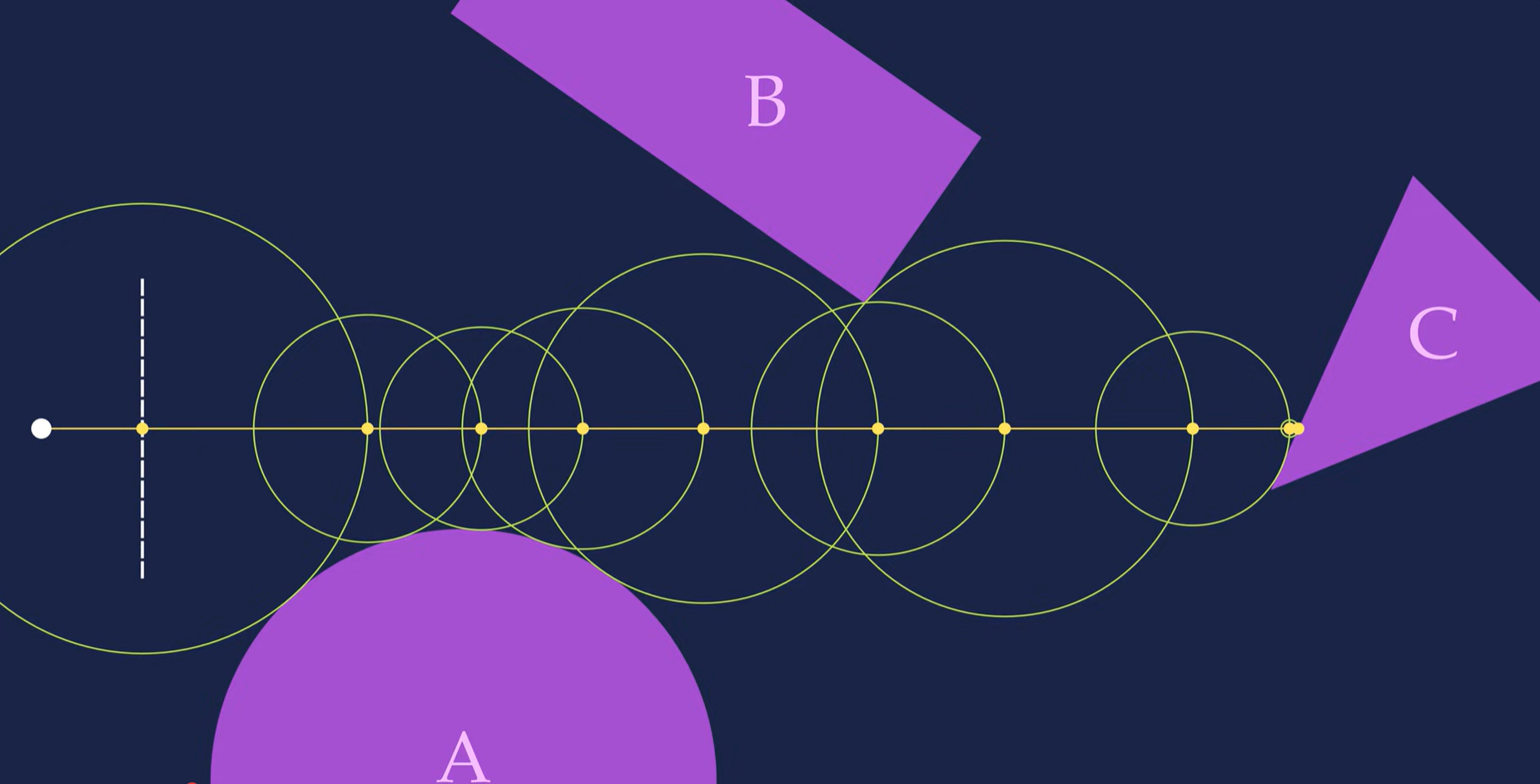Raymarching & SDF illustration, (Source: Youtube - Sum and Product)

Finally, note that since the SDF tells us the distance to the closest object, we can also use it to determine when to stop marching. We simply set some very small threshold, and then once the minimum SDF value is lower than that threshold, we say that we’ve “hit” the closest object!

Now, we can leverage the combined use of raymarching and SDFs to construct a scene.

Constructing the Scene

With raymarching ready, constructing the scene is simple.

For each shape we want to add, we add its SDF to a list of SDFs for each object in the scene. Then, we create a function called map() that will take a 3D position, calculate the SDF value for all objects at that position, and then return two things:

The distance to the closest object
Information about the closest object

This way, if we reach the “stop” threshold (i.e. the distance becomes small enough), we will know which object that we “hit”. We can then use information about that object to pick the color of the pixel that the ray was marched through.

For example, I could take the color (referred to as the albedo) of this object and simply set the value of the pixel to that color, and this would give me a simple unlit scene. 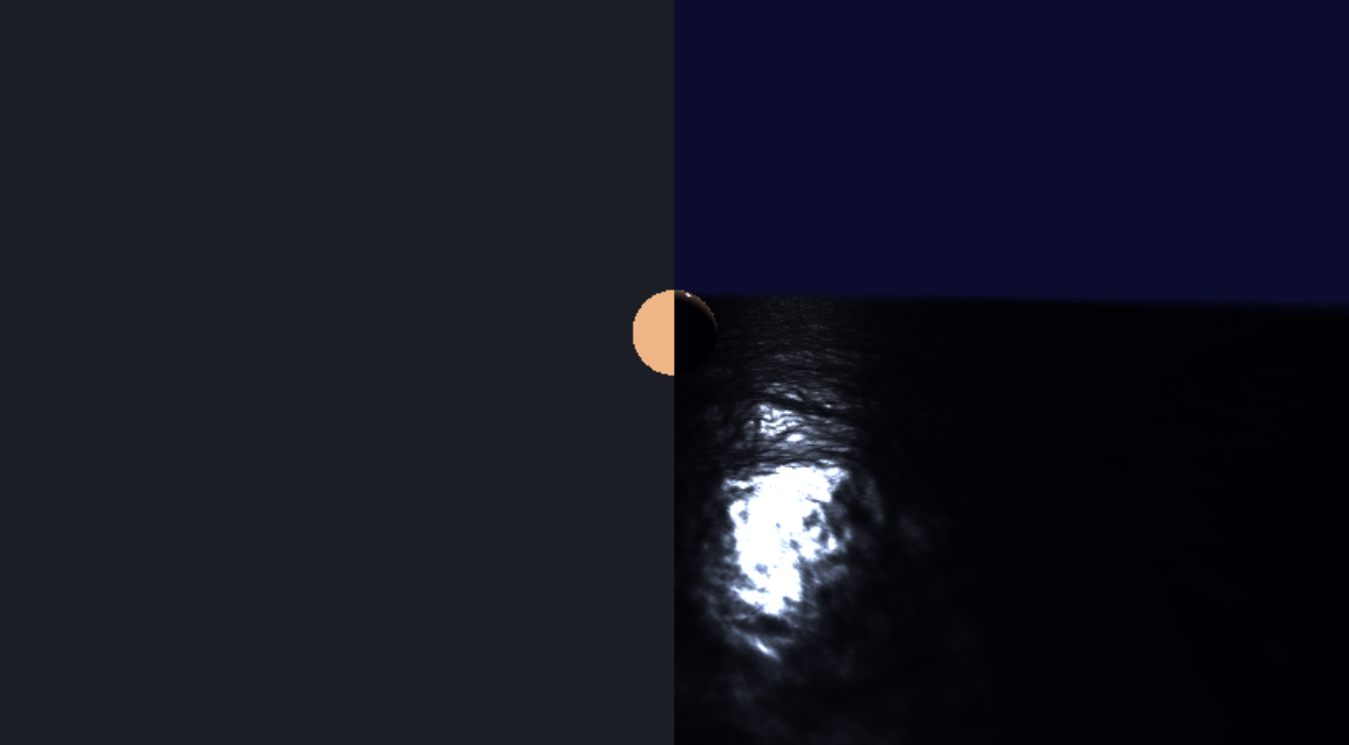A half-unlit-half-lit raymarched scene. The left half is rendered by setting the pixel’s color to the albedo of the object. The right half is rendered using lighting calculations.

Of course, for a better looking scene, we should do much more than simply use the albedo directly.

Lighting Calculations

By using raymarching as described above, we are now able to determine which object surface is seen at each pixel. With this, we can take information about this surface to determine what color should be seen at this pixel.

Remember, the ultimate goal is mapping the pixel position (fragCoord) to the color that should be at that pixel (fragColor). So far, we’ve mapped our pixel position to the surface that will be rendered at the pixel. Now, we want to map the information about that surface to our final pixel color.

Input Data

For lighting calculations, we would want the following information about a surface:

The surface’s albedo. This can be thought of as the surface’s underlying color.

In a physics context, it represents the color of diffuse reflection from this surface. That is, what color is a light ray that is absorbed and re-emitted by this surface?
The surface’s roughness. This is, literally, how rough a surface is. The rougher a surface, the more reflected light “spreads out”, giving it a more “flat” look, like plastic or drywall. The less rough a surface, the more “glossy” or “shiny” it looks, closer to a polished or wet surface, or a mirror.

More specifically, this relates to the microfacet model of surfaces. A higher roughness implies a higher likelihood of some microfacet deviating from the macrosurface normal. The more microfacets deviate, the less likely light will reflect perfectly on the macrosurface.
The surface normal. This is a vector that points perpendicular to the surface. This essentially tells us in which direction a surface is “facing”, which can derive a lot of information on how that surface is lit.
The surface’s metallic value. Metallic surfaces (e.g. silver) do not reflect light diffusely, giving them their characteristic appearance. This is as opposed to dielectric surfaces (e.g. wood), which do reflect light diffusely, and are generally more common. Thus, to render metallic surfaces, we must have the option to disable diffuse reflection, which is what this provides. The surface color is interpolated between dielectric (diffuse included) and metallic (diffuse excluded) lighting using this value.

In reality, a surface is either metallic (metallic = 1) or not (metallic = 0). However, we allow any value in between as an artistic choice for semi-metallic materials.

Additionally, we’d like some information about this surface’s relation to the scene:

The view direction, denoted \(\mathbf{v}\). That is, the direction from the point on the surface that we’re rendering, to the camera.
The light direction, denoted \(\mathbf{l}\). That is, the direction to the light source.

For simplicity, we’ll do shading calculations once for each light source in the scene, and then add up all of the results to get our final color.

Shading

With this data available to us, we can now calculate the final color of that surface, and thus in turn, of this pixel. While there are several different possible shading models, we are going to use a variant of physically based rendering (PBR). This is a type of rendering that is derived from physical models of how light interacts with a surface, the goal being to create an image that is as realistic as possible.

Note this is also going to be a simplified explanation. For more details, I recommend this article on LearnOpenGL by Joey de Vries, and these course notes by Naty Hoffman

Briefly returning to reality, note that if we can see a surface, it implies that light from some light source has hit that surface and then has been re-emitted in some way toward our eyes. We assume this re-emission can happen in one of two ways:

Diffuse: The ray of light is absorbed by the surface and re-emitted in all directions. This is a “flat” type of lighting, where changing the position of your eyes doesn’t effect the color you see at that position on the surface. The color that as re-emitted is the albedo of the surface. That is, an aggregate of the wavelengths of light that the surface does not absorb.
Specular: The ray of light is reflected from the surface, re-emitted in a single direction. This is the “shiny” type of lighting. Prime examples of specular light are metals and mirrors. What you see on a mirror depends heavily on where you’re standing. This is because the ray of light reflects in a direction that is dependent on the surface normal and incoming direction. Thus, the ray you see depends on in which direction you’re in from the surface’s perspective.

With this assumption, we can now independently calculate the diffuse and specular components of the light emitted from a surface, and then add them together to get our final color.

Diffuse

Of the two, diffuse lighting is easiest to calculate. This is because it is a result of light being absorbed and emitted equally in all directions. Since it is emitted equally in all directions, the diffuse lighting that can be seen on a surface does not vary by viewing position.

To calculate diffuse lighting, we need only two quantities: the normal direction and the light direction, denoted \(\mathbf{n}\) and \(\mathbf{l}\) respectively. The more these two align, the stronger the diffuse lighting is.

This can be intuitively seen by thinking of a flat surface. The more that this surface “faces” the light source, the brighter that surface will be. Additionally, we consider this brightened color to be “the color” of the surface.

To calculate diffuse lighting, we use the following formula:

\[L_d=(\mathbf{n} \cdot \mathbf{l})L_ik_d\frac{c}{\pi}\]

Where \(L_d\) is outgoing diffuse light, \(L_i\) is incoming light from the light source, \(k_d\) is the diffuse lighting coefficient, and \(c\) is albedo.

Note the division by \(\pi\). This is done for energy conservation, as the incoming light is distributed equally in all directions, and thus the intensity of the light seen will be lower than the incoming light at the surface.

There is also a multiplication by \(k_d\). This represents the portion of the incoming light that is reflected diffusely. Since whether or not a single ray of light is reflected or absorbed is a stochastic process, we represent both cases with this coefficient and its complement \(k_s\).

Finally, we multiply by \(\mathbf{n} \cdot \mathbf{l}\) to scale the intensity of the incoming light by how much the normal aligns with the light direction. This quantity is also equivalent to \(\cos(\theta)\), where \(\theta\) is the angle between \(\mathbf{n}\) and \(\mathbf{l}\). At an angle of \(0\), all of the incoming light is received. As the angle grows, less and less of it is received, and thus the incoming light is scaled down accordingly.

Specular

Specular lighting, as compared to diffuse, is more involved. To determine the specular light seen at a point on a surface, we model our surface using the microfacet model.

Briefly, the microfacet model assumes that a surface is made up of infinitesimally small perfectly reflective mirrors. Then, the roughness parameter describes the variance of the normal of any one microfacet from the macrosurface’s normal (that is, the normal of the aggregate surface we are rendering, \(\mathbf{n}\)).

With a lower roughness, more microfacets will be aligned with the macrosurface, and the macrosurface will behave more closely to a mirror (i.e. a perfectly reflective surface). With a higher roughness, more microfacets are misaligned, and light from several incoming directions is reflected toward the camera, creating a more “spread out” reflection. 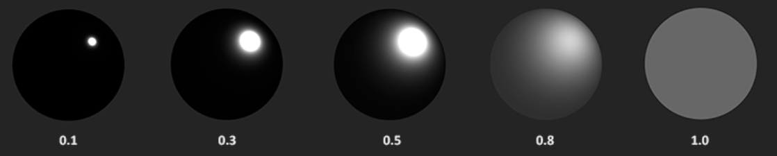Roughness visualization (Source: LearnOpenGL)

Now, consider some perfectly reflective surface, and a ray of light hitting that surface. Denote the direction to the source of the light as \(\mathbf{i}\), and the surface normal as \(\mathbf{n}\). We know that the outgoing direction of the reflected light \(\mathbf{o}\), has the property that the angle between \(\mathbf{i}\) and \(\mathbf{n}\) is the same as the angle between \(\mathbf{o}\) and \(\mathbf{n}\). This is because reflection involves inverting the component of a vector parallel to the normal of a surface. As a result, the components of \(\mathbf{i}\) and \(\mathbf{o}\) parallel to the surface are additive inverses of each other.

Thus, we know that \(\mathbf{i} + \mathbf{o}\) would cancel out this parallel component, and we’d be left with a vector aligned with the surface normal. Normalize this vector, and we get what we call the halfway direction, denoted \(\mathbf{h}\). ![]images/Pasted image 20260125110941.png) Halfway direction visualization (Source: LearnOpenGL)

\(\mathbf{h}\) tells us, for some \(\mathbf{i}\) and \(\mathbf{o}\), what direction the surface normal must be for light coming from \(\mathbf{i}\) to reflect in the direction \(\mathbf{o}\).

In our case, we have a light source and a camera. Thus, our incoming direction is \(\mathbf{i}=\mathbf{l}\), and our outgoing direction is \(\mathbf{o}=\mathbf{v}\) (\(\mathbf{v}\) is view direction). We then calculate \(\mathbf{h}\) as

\[\mathbf{h} = \frac{\mathbf{v}+\mathbf{l}}{||\mathbf{v}+\mathbf{l}||}\]

From this, we now know that if the surface was perfectly reflective, the reflected light would only be seen by the camera if \(\mathbf{n} = \mathbf{h}\). However, for rougher surfaces, \(\mathbf{h}\) is more of a suggestive factor, where the closer it is to \(\mathbf{n}\), the stronger the specular reflection is.

This is because the most probable normal of a microfacet is the macrosurface normal. For higher misalignments from the normal direction, less and less microfacets are so misaligned. Thus, you get the strongest specular reflection from light when \(\mathbf{h}\) and \(\mathbf{n}\) are the same, and then the reflection weakens gradually as \(\mathbf{h}\) and \(\mathbf{n}\) differ more.

In essence, roughness dictates how fast the specular reflection weakens as \(\mathbf{n}\) differs from \(\mathbf{h}\). The faster it weakens, the smaller the “specular lobe” is. Additionally, due to conservation of energy, smaller specular lobes will have a higher intensity, appearing brighter, since the light is less widely distributed.

The Specular BRDF

Now, using these principles, we must somehow calculate the exact portion of the incoming light that is reflected. Fortunately, research has been done on creating a function that tells us just that, and we call it the Bidirectional Reflectance Distribution Function (BRDF).

In actuality, a full BRDF contains both the diffuse and specular components, as it determines the total portion of incoming light (more accurately, radiance) that is re-emitted in a specific direction. The Cook-Torrance BRDF is as follows:

\[f_r(p,\omega_i,\omega_o) = \frac{DGF}{4(\mathbf{i} \cdot \mathbf{n})(\mathbf{o} \cdot \mathbf{n})}\]

Where \(D\), \(G\) and \(F\) are the Distribution, Geometry and Fresnel terms, respectively.

Was going to explain BRDF here but this is going way too deep. OpenGL does a good coverage, the GGX paper explains it in depth very well, and this paper is a great resource for the G term

Water

Now we switch the plane for a heightmap.
We can use perlin noise with some amplitude for a varying heightmap, but there’s weird gaps in it.
Normals
This is because the ray still uses the height difference for the SDF, but it may be closer since it’s oblivious to slope difference and thus if something is “in front” of it and closer than the y axis difference. As a result, it may go “through” the water plane and not hit anything at all as if there’s nothing there.
This can be fixed by approximating the normal of the heightmap by sampling a tetrahedron around the point Then, you use the normal to approximate the closest point using a linear approximation with the height difference just below, and then multiply that by a safety factor (0.5 in my case) just incase the linear approximation is too large still.
This works, and there’s no longer gaps, and it also allows for accurate lighting but we want to use different h values for different normal detail levels, so we separate the sdf normal h value and the lighting normal h value (the one assigned to the “hit” object)
Waves
Now we want something that looks like waves, for this, we overlap several perlin noise samples and then vary the texture coordinate with time, making the tex coord vary on the 2D plane in different directions.
Some of the perlin noise maps we further multiply by a sine wave to make it actually “wavy”.
Combining this with a metallic material, this makes it look like an actual liquid

Bugs

Water looked dumb but realized that the roughness value was too high, looked too plasticky but now is better when barely rough and very metallic. Note water is a near-perfect specular reflector, so metallic is accurate.
Needed to experiment with the h value to make it look right, different values made the water look “flatter”
At low roughness, the specular highlight was too dim, but this was because the D value capped by maxing the denom with epsilon, so created a second epsilon that is smaller to allow for less rough shapes to look correct.

Ended up with this result: